Abstract
Heavy-tailed distributions are increasingly found to better fit empirical data in engineering, finance, physics, network science, and related fields. Among them, -stable distributions play a central role being limiting laws in the generalized central limit theorem: they are expected to be exceptionally good models whenever sums of multiple independent heavy-tailed sources are at play. Despite their theoretical importance, their practical use remains challenging: -stable probability densities generally do not have closed-form expressions, and numerical evaluation and random variate generation can be difficult, especially in the multivariate setting. This paper presents AUB-HTP, a Python package for numerical computation and simulation of -stable distributions. The package provides scalar density evaluation using several complementary methods, including Zolotarev-type integral representations, series formulas, and numerical inversion of characteristic functions. It also provides random variate generation for scalar and multivariate -stable distributions, with support for flexible spectral measures through LePage series representations. Numerical experiments demonstrate that AUB-HTP improves the accuracy, stability, and parameter coverage of existing tools for scalar density computation, while adding new capabilities for multivariate simulation. The package is designed to support reproducible computational work involving heavy-tailed models across a broad range of scientific applications.
1Introduction
Heavy-tailed distributions arise naturally in many scientific and engineering applications, including communications, signal processing, finance, physics, and network modeling Nassar et al. (2008)Tsihrintzis et al. (1995)Crovella et al. (1998)Nolan (2013)Taleb (2022). In such settings, rare but large deviations occur more frequently than predicted by light-tailed models such as the Gaussian distribution. As a result, Gaussian-based modeling can significantly underestimate the probability and impact of extreme events.
Among heavy-tailed models, -stable distributions occupy a central theoretical position. They generalize the Gaussian distribution through the stability property: sums of independent -stable random variables remain -stable, up to location and scale changes. They also arise as limiting distributions for normalized sums of independent random variables under the generalized central limit theorem B. V. Gnedenko and A. N. Kolmogorov (1968). These properties make -stable laws natural candidates for modeling aggregate effects generated by many independent heavy-tailed sources.
A major practical limitation of -stable distributions is that their probability density functions (PDF)s generally do not admit closed-form expressions, except in the special cases of the Cauchy and Lévy distributions. Consequently, numerical tools are required for density evaluation, modeling, and simulation. Existing approaches for scalar -stable random variate generation, such as the Chambers–Mallows–Stuck (CMS) method Chambers et al. (1976), are well established, but they do not directly address general multivariate -stable distributions. In the multivariate case, available simulation methods typically focus on special spectral measures, such as isotropic or sub-Gaussian models Nolan (2013), rather than arbitrary spectral measures.
This paper presents AUB-HTP, a Python package for computational work with -stable distributions. The package provides scalar density computation using several numerical methods, including Zolotarev integral representations Zolotarev (1986), Skorohod-Pollard-Bergström formulas A. V. Skorohod (1961)Pollard (1946)Bergström (1952), and direct numerical inversion of the characteristic function[1]. These methods provide complementary tradeoffs in terms of accuracy, speed, and robustness across parameter regimes. In addition, AUB-HTP implements random variate generation for scalar and multivariate -stable distributions. For the multivariate case, the package uses LePage series representations LePage et al. (1981), which support flexible spectral measures and perform particularly well in challenging heavy-tailed regimes, including small values of .
The goal of AUB-HTP is to make -stable modeling more accessible to computational scientists by providing reliable density evaluation, flexible simulation tools, and reproducible numerical routines within the Python ecosystem. The main contributions of this work are: (i) a unified Python implementation of several scalar -stable PDF evaluation methods; (ii) a flexible random variate generator for scalar and multivariate -stable distributions; (iii) support for general spectral measures through LePage series; and (iv) numerical benchmarks comparing accuracy, runtime, and robustness against existing implementations.
Notations
We adopt the following conventions. The vector represents a column vector and is its transpose. The Euclidean inner product of two vectors and is denoted by and the norm of by . The unit sphere in is denoted by . The class of all borel subsets in a metric space is represented by . We use to indicate that the two random vectors and are independent. When a random vector is distributed uniformly on the unit sphere, we write . For a random variable that is Gamma distributed, we write , and we use the following parameterization for the PDF
where is the Gamma function.
2Preliminaries on -Stable Distributions
We adopt the definition of a multivariate stable vector given in Samorodnitsky & Taqqu (2000):
In particular, we are interested in -stable [2] random vectors.
In the scalar case () –and whenever , the spectral measure boils down to two mass points on , and the characteristic function in (2) is expressible in terms of 4 parameters: the stability index , skewness , scale , and location . In this case, we denote an -stable random variable using the same notation as in Nolan Nolan (2020), where is the parameterization index (or type). We will use the symbols and to refer to the two common type-0 and type-1 parameterization, respectively. In the multivariate case, we denote a -dimension non-degenerate -stable random vector with stability index , spectral measure and shift vector , by . Note that Definition 2 corresponds to the generalization of the scalar case under the parameterization .
Parameterizations of scalar -stable distributions
There two parameterizations and differ primarily in how they define the location (shift) of the distribution, particularly near . For a given and , let be a “standard" -stable variable corresponding to and .
Parameterization 0:
A random variable if
The characteristic function of is given by
This parameterization has the advantage of avoiding discontinuities near by adjusting the shift behavior. It is often preferred for numerical stability Nolan (2020).
Parameterization 1:
A random variable if:
with a corresponding characteristic function given by
Unlike type-0, this parameterization requires an explicit adjustment to the location when .
Note that the choice of parameterization directly affects the shift and symmetry of the distribution, especially when and is close to 1. In both forms, the distribution can be standardized by setting and , in which case we use the abbreviations and respectively.
In the univariate case, our package can simulate both parameterizations .
3Scalar Density Evaluation
The AUB-HTP package provides numerical evaluation of scalar -stable probability density functions through a SciPy-like interface. This component complements the random number generator: the generator produces samples, while the density module provides the reference curve used for model verification, visualization, and numerical comparison.
Except for Cauchy and Levy laws, -stable distributions do not have a closed-form density, which must therefore be computed using numerical inversion or analytic representations that are valid in specific parameter regions.
Towards fulfilling our main objective of reducing expensive quadrature calls while preserving accuracy across a wide range of , , and sample values, the density evaluator combines three methods:
direct inversion of Nolan’s characteristic function near the mode Nolan (2020)
Zolotarev’s integral representation in the middle range Zolotarev (1986)
Skorohod-Pollard-Bergström’s series expansions in the tails A. V. Skorohod (1961)Wintner (1941)Pollard (1946).
3.1Input standardization
All density calls are first mapped to a standardized variable allowing the internal routines to work on standardized densities while still supporting user-facing location and scale parameters. More specifically, given an input sample value the code evaluates
then rescales the final density by . For the parameterization for example, the shift is given by Nolan (2020, equation 1.5)
as can be deduced from equation (5).
Additionally, if is the PDF of a normalized -stable random variable, for negative evaluation points the code uses the symmetry relation Nolan (2020, proposition 1.1)
and most formulas only need to be evaluated on the positive half-line.
3.2Hybrid evaluation strategy
The main density function acts as a dispatcher. It divides the input array into regions and applies the method that is most accurate for each region.
For small (see equation (7)), the package uses direct inversion of the characteristic function. While this method is slower than the series expansions, it is stable near the mode where tail formulas are not accurate.
For intermediate values of , the package uses Zolotarev’s integral representation. This provides a useful compromise between direct inversion and asymptotic series methods.
For large , the package uses Skorohod-Pollard-Bergström series’ expansions. These formulas are fast in the tails and avoid repeated numerical integration.
The switching points between methods are not fixed constants. They are instead selected from precomputed cutoff functions depending on . These cutoffs were obtained using grid-based comparison with scipy.stats.levy_stable.pdf. At runtime, the code queries the corresponding cutoff and applies Boolean masks to route each input point to the selected method.
Density formulas
For direct inversion in the parameterization Nolan (2020), the density is computed from the characteristic function. The standardized density is
These integrals are evaluated with scipy.integrate.quad_vec.
For the middle region, the code uses Zolotarev’s integral representation Zolotarev (1986). For and ,
where
and where is evaluated following Zolotarev’s formula Zolotarev (1986). This integral is computed using the function scipy.integrate.quad.
For the tail region, we use Skorohod-type series expansions A. V. Skorohod (1961)Wintner (1941)Pollard (1946) of the form
where
The number of terms used to calculate the series is appropriately chosen depending on the parameter range. In the current package, the branch uses a larger truncation level, while the branch requires fewer terms in the tested regimes.
3.3Validation
The density evaluator was tested against scipy.stats.levy_stable.pdf on grids of , , and . The near-mode tests used , while the tail tests examined values up to .
The comparison recorded the following metrics:
Maximum absolute error:
Maximum relative error:
where prevents division by zero.
Mean absolute error:
Runtime against SciPy, reported through the speedup factor:
The tests show close agreement across most of the parameter space, but they also reveal regions where the SciPy reference exhibits irregular numerical behavior. The strongest agreement occurs away from the narrow region around , where changes in the parameterization and the presence of logarithmic terms make density evaluation more sensitive. In this region, visual diagnostics are important because the relative difference may become large when the reference density is close to zero or numerically unstable. Figure 1 illustrates this behavior near using the maximum relative difference measured around the mode. Away from , Figure 1 shows agreement with the SciPy reference. Results for the remaining error metrics, parameter ranges, and tail evaluations, together with the complete benchmark data, are available in the Github repository[3].
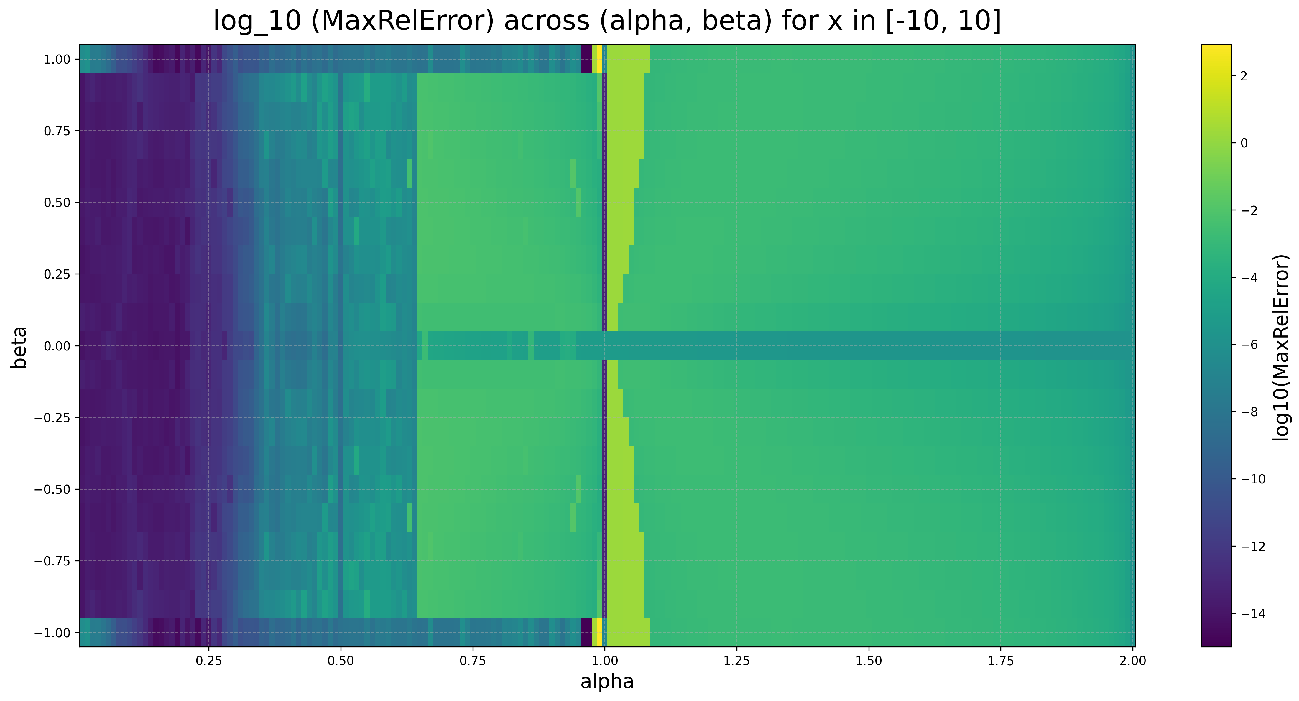
Figure 1:Maximum relative difference across near the mode. Larger values near mark the most sensitive numerical region.
3.4Discrepancies in the SciPy reference
While scipy.stats.levy_stable.pdf The SciPy Community (2026) is used as the main numerical reference, we observed that it has some discrepancies for certain parameter values. These discrepancies appear mostly near the sensitive region around , and they can create misleading relative difference values.
The main issue is that the SciPy PDF sometimes shows unusual zero or near-zero regions in some places while the densities are known to be smooth. Since the maximum relative difference contains a division by the reference value, even a small disagreement in such regions can produce a very large relative difference. Therefore, some of the large relative differences in the benchmark tables do not necessarily mean that our PDF generator is inaccurate. Instead, they are likely due to the instability or discontinuity in the reference PDF.
To validate this, we generated visual diagnostic plots comparing the AUB-HTP with the levy_stable PDF values. Figure 2 shows several cases where the SciPy reference generates unexpected zero windows or sharp changes, while the PDF generated using our package remains smooth.
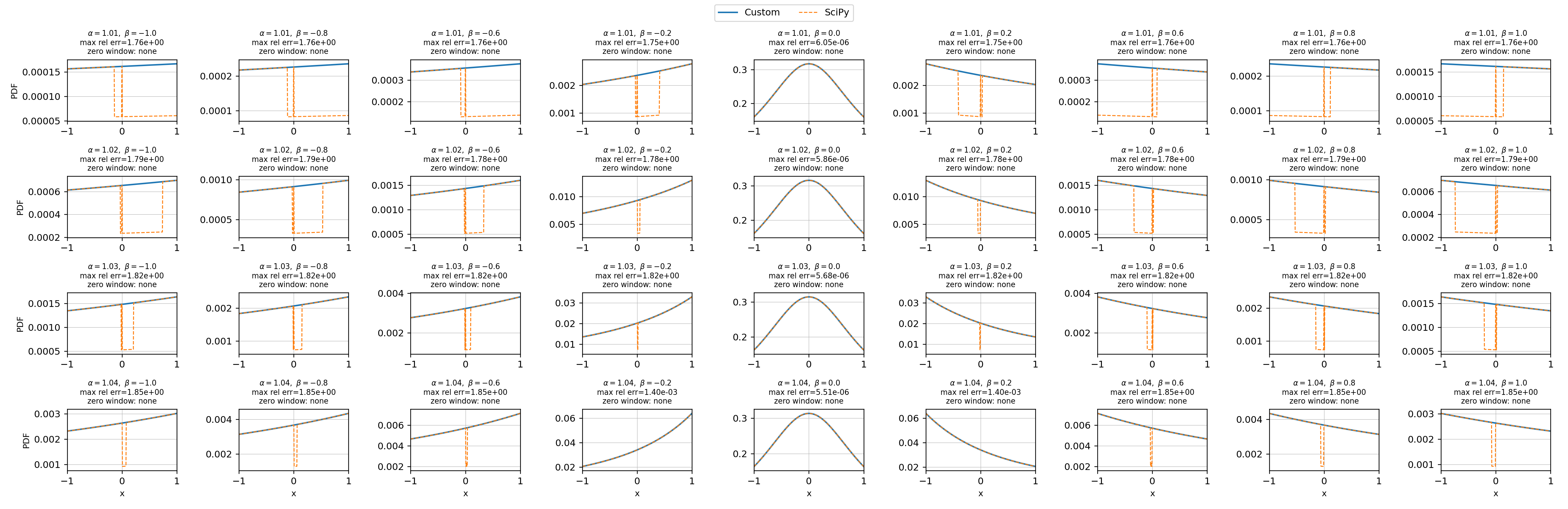
Figure 2:Visual comparison between AUB-HTP PDF generator and scipy.stats.levy_stable.pdf. The plots zoom into regions where the SciPy reference becomes numerically zero or behaves irregularly. These regions explain why some relative difference values become large even when our generated density remains smooth.
The heatmaps are useful for locating sensitive parameter regions, but the diagnostic plots were needed to understand whether the difference is primarily attributed to our method or the numerical reference.
3.5Runtime
The adopted hybrid strategy reduces runtime by avoiding direct quadrature when a faster formula is accurate enough. The largest gains occur in the tail region, where series expansions replace repeated numerical integration.
In the benchmark runs, the median speedup was approximately , with larger speedups in tail-heavy evaluations. These gains come from three design choices:
vectorized array operations
region-specific method dispatch
reuse of precomputed cutoff functions.
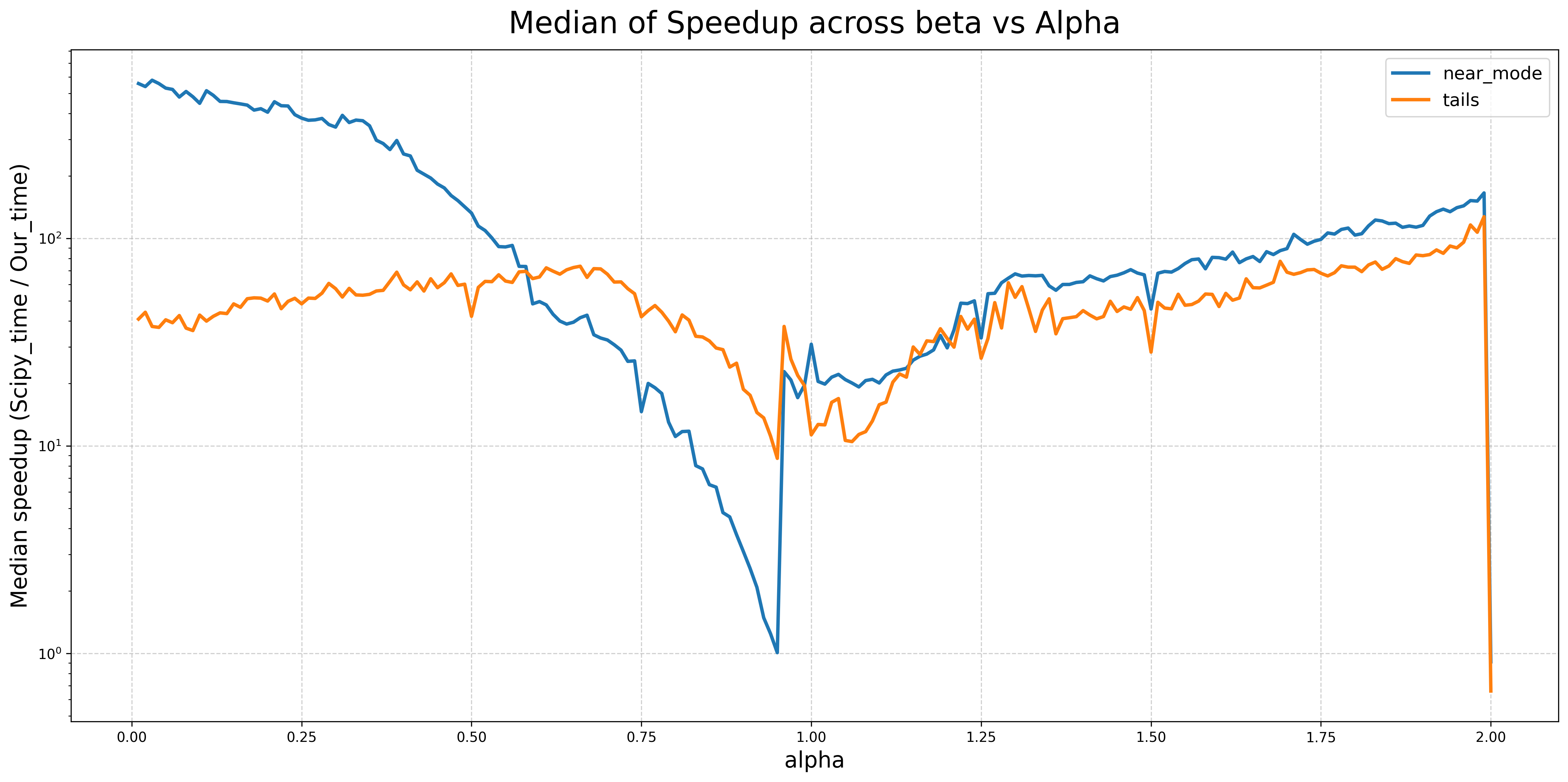
Figure 3:Median runtime speedup relative to scipy.stats.levy_stable.pdf. The largest gains occur where the series expansions are selected.
The speedup plot in Figure 3 shows that our method is strictly faster than scipy.stats.levy_stable.pdf for almost all tested values of . Note that the vertical axis is on a logarithmic scale and values between 10 and 100 represent large runtime improvements. For small values of , especially in the near-mode range, the speedup is very high. This is because the method selection avoids unnecessary numerical integration and uses the formulas that are faster in those regions. In the tail range, the speedup is also consistent for most values of , since the Skorohod-Pollard-Bergström formulas replace repeated quadrature calls. The smallest speedups occur near which is expected since this region is numerically delicate. The formulas change around , and the characteristic function contains a logarithmic correction term. The package therefore relies more on direct inversion in this region, which is slower than the series-based methods.
4Generating -Stable Random Vectors
In the univariate case, the package implements a numerically stable version of the Chambers, Mallows, and Stuck method which is presented in Chambers et al. (1976)Nolan (2020). In the multivariate setup, the proposed random number generator is based on a theoretical foundation that we state next.
4.1The LePage series
The LePage series Samorodnitsky & Taqqu (2000) was first introduced in LePage et al. (1981) and allows for simulating a multivariate stable vector with a stability index and a given spectral measure through the use of the following theorem Bentkus et al. (2001, Theorem 4)
Theorem 1 indicates that sampling a multivariate stable vector can be done by computing the truncated series as in equation (20). Since the vector resulting from the series has a zero shift vector Bentkus et al. (2001, Remark 1), we simply add after sampling using the LePage series, when needed. The analysis of the truncation error is deferred to Appendix 7.
In the following section, we present algorithms to sample according to well-known spectral measures, namely: Isotropic, Sub-Gaussian, Discrete, and Mixed spectral measures.
4.2Common spectral measures
4.2.1Discrete spectral measures
In the case of a discrete spectral measure with mass points, we store the point masses in an array and draw randomly with the probability of each vector being
4.2.2Isotropic spectral measures
For an isotropic spectral measure, we sample the vectors uniformly on . To this end, several algorithms are available and we refer the reader to Schnabel & Janke (2022) where various such algorithms are discussed. In our computations, we adopt the method presented in Muller (1959) due to its simplicity and computational efficiency. Our package sets the spectral measure of the sphere to 1, and then scales the truncated LePage series by an appropriate factor to adjust for the desired scale given by the user: When the spectral measure of the sphere is 1, it can be verified that the characteristic function is given by
To achieve a scale , we therefore multiply the truncated series by
4.2.3Sub-Gaussian (elliptical) spectral measures
A sub-Gaussian random vector is characterized by a positive-definite shape matrix . If is a unit-scale isotropic multivariate stable random vector with stability index then is a sub-Gaussian random vector with shape matrix where is the Cholesky decomposition of Nolan (2013). As such, to sample from , one can first sample a unit-scale isotropic random vector with the same stability index using the LePage series as in Section 4.2.2 and multiply it by the Cholesky decomposition of . In section 7.2 in the appendix, we analyze the resulting Mean Square Error (MSE) of .
A useful alternative would be to sample the vectors for the sub-Gaussian case by sampling vectors uniformly distributed on the unit sphere and multiplying them by . Indeed, if is the -terms LePage series, by Theorem 1, converges in total variation to , and
converges in total variation to , which is the desired sub-Gaussian random vector.
The package first samples and then computes the sum presented in (25) to sample a sub-Gaussian random vector .
4.2.4Mixed spectral measures
Now consider the scenario where the spectral measure at hand is a mixture of different spectral measures: . If are their respective associated weights, the mixed spectral measure is given by
To sample from this spectral measure, we proceed as follows.
For each weight we associate its corresponding probability as
Then, we sort the probabilities in non-decreasing order that we assume –without loss of generality– to be hereafter.
We draw ,
If sample from ,
else if , sample from ,
else iterate on the remaining spectral measures.
This algorithm achieves a sampling from the mixture of with probabilities respectively.
5Implementation
Whenever the LePage series is used, the package chooses the number of terms to achieve an MSE less than 0.01 using Theorem 2 in Appendix 7. This number is capped at 50,000 terms and a warning is issued whenever this cap is reached.
5.1Univariate random number generator
In the univariate case, the software samples , and the type 1 parameterization is used by default.
import aub_htp as ht
alpha=1
beta=0
loc=0
scale=1
n=500000
samples=ht.alpha_stable.rvs(alpha=alpha, beta=beta, loc=loc, scale=scale, size=n)
In Figure 4, we present some examples where univariate -stable variables were sampled using our implementation, and plot the truncated histogram of values. Each histogram is overlayed by the pdf values which are computed using the SciPy levy_stable numerical package.
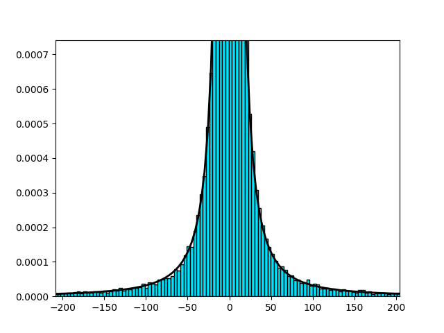
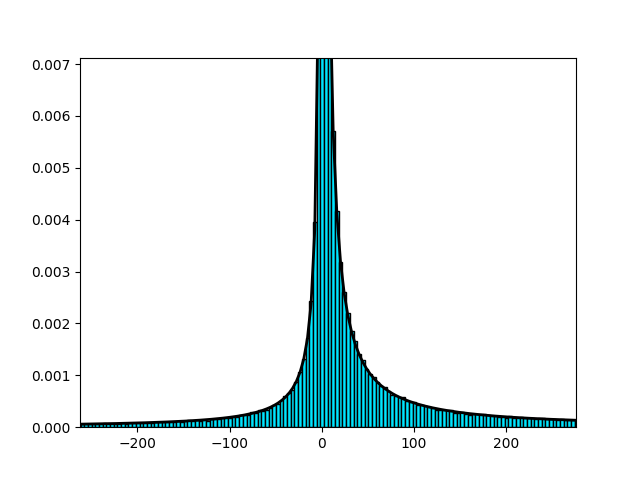
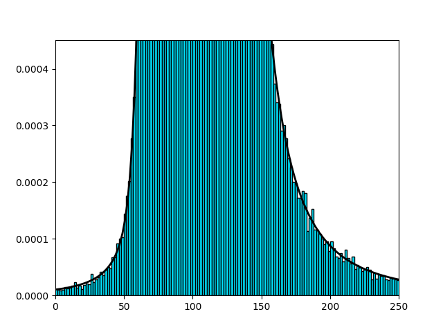
Figure 4:Truncated histogram of -stable distributions, each containing points.
An example using the type 0 parameterization is presented in Figure 5.
import aub_htp as ht
alpha=0.1
beta=1
loc=-500
scale=10
n=500000
ht.alpha_stable.with_parameterization("S0")
samples=ht.alpha_stable.rvs(alpha=alpha, beta=beta, loc=loc, scale=scale, size=n )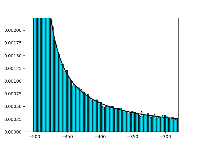
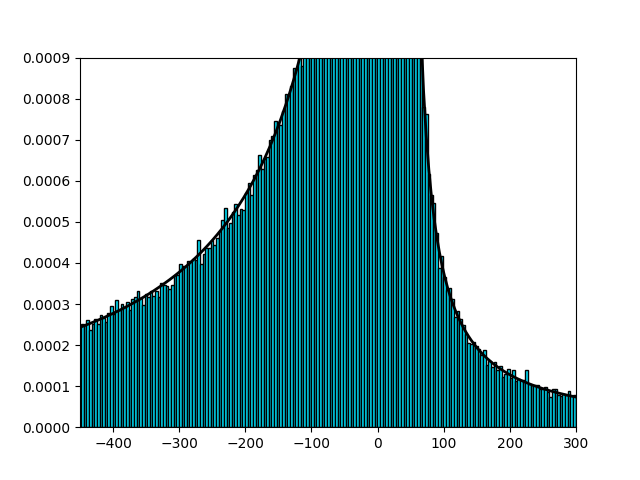
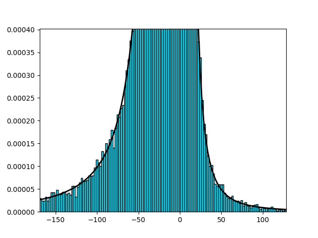
Figure 5:Truncated histogram of -stable distributions, each containing points.
5.2Multivariate random number generator
5.2.0.1Isotropic -stable random vector:
An isotropic -stable random vector with characteristic function
can be generated using the AUB-HTP package as follows:
import aub_htp as ht
from aub_htp.random import IsotropicSampler
alpha = 0.5
gamma = 1
shift= [0,0]
d = 2
n=500000
sampler = IsotropicSampler(number_of_dimensions= d, alpha = alpha, gamma = gamma)
samples = ht.multivariate_alpha_stable.rvs(alpha = alpha, spectral_measure_sampler = sampler,shift=shift, size = n)
where is the stability index, is the scale parameter and represents the shift vector. Figure 6 depicts scatter plots of the generated isotropic -stable random vectors.
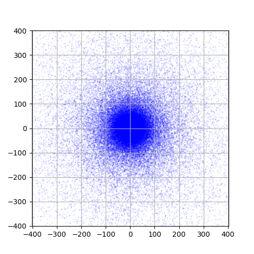
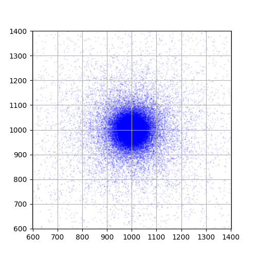
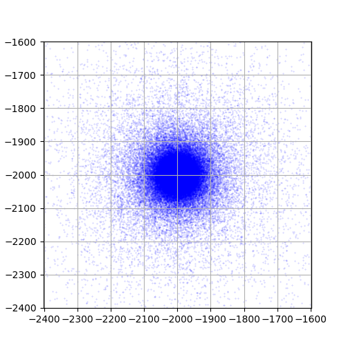
Figure 6:Scatter plots each containing points of isotropic -stable distributions. The plots have been truncated to a range of 400 points within the shift vector.
5.2.0.2Elliptic -stable random vector:
An elliptic -stable random vector with shape matrix with the following characteristic function
can also be generated using AUB-HTP. We note that the elliptic sampler takes the total mass of the unit sphere as input. If the total mass of the sphere is not specified, the software estimates it using Monte Carlo simulations (with 106 samples) as follows:
where the equality is due to Samorodnitsky & Taqqu (2000, proposition 2.5.8), and where are i.i.d. samples according to . Equation (30) is justified by the application of the Weak Law of Large Numbers (WLLN) because the random variable has a finite second moment. Indeed,
where equality is due to the Cholesky decomposition definition and in we used the -weighted norm . Finally, the inequality in is due to the fact that where is the largest eigenvalue of , equal to the norm of matrix Horn & Johnson (1985).
Finally, we note that the MSE resulting from estimating the total mass of the sphere using equation (30) is given by Niederreiter (1992, Theorem 1.1).
An example code is as follows.
import aub_htp as ht
from aub_htp.random import EllipticSampler
alpha = 0.5
shift= [0,0]
d = 2
n=500000
sigma1=[[2,0.8],[0.8,1.5]]
sampler =EllipticSampler(number_of_dimensions = 2, alpha = alpha, sigma = sigma1)
samples = ht.multivariate_alpha_stable.rvs(alpha = alpha, spectral_measure_sampler = sampler,shift=shift, size = n)
Figure 7 shows the scatter plots of the elliptical -stable random vector, where we use the following shape matrices
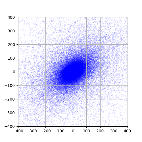
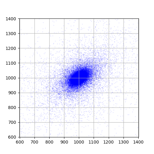
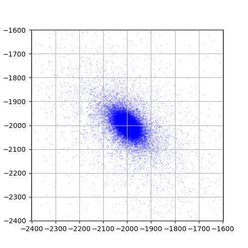
Figure 7:Scatter plots each containing points of elliptic contoured -stable distributions; the plots have been truncated to a range of 400 points within the shift vector.
5.2.0.3Discrete spectral measures:
For an -stable random vector that has a discrete spectral measure with point masses at positions and corresponding weights , the corresponding characteristic function is given by
Such a vector can be generated as follows:
import aub_htp as ht
from aub_htp.random import DiscreteSampler
alpha = 0.2
shift= [0,0]
d = 2
n=500000
positions=[[1,0],[0,1],[-1,0],[0,-1]]
weights=[1,1,1,1]
sampler = DiscreteSampler(alpha = alpha, positions = positions,  weights = weights)
samples = ht.multivariate_alpha_stable.rvs(alpha = alpha, spectral_measure_sampler = sampler,shift=shift, size = n)
with corresponding scatter plots shown in Figure 8.
![\text{Masses}=[1,1,1,1], \text{weights}=[(1,0),(0,1),(-1,0),(0,-1)], \alpha=0.2, \boldsymbol{\mu}^{0 T}=(0,0).](/scipy_proceedings/build/Figure_10-3b02ce29a77c3a9314e40c686a5a39c1.png)
(a), .
![\text{Masses}=[\frac{1}{4},\frac{1}{4},\frac{1}{4},\frac{1}{4}], \text{weights}=[(1,0),(0,1),(-1,0),(0,-1)], \alpha = 1.2, \boldsymbol{\mu}^{0 T}=(1000,1000).](/scipy_proceedings/build/Figure_11-c91b403820197b7993be7fba04f86243.png)
(b), .
![Masses =[\frac{1}{5},\frac{1}{5},\frac{1}{5},\frac{1}{5},\frac{1}{5}], weights =[(1,0),(0,1),(-1,0),(\cos(\theta),-\sin(\theta)), (\cos(\pi - \theta),-\sin(\pi - \theta))], \theta = \frac{13\pi}{20}, \alpha=0.1, \boldsymbol{\mu}^{0T}=(0,0).](/scipy_proceedings/build/Figure_12-6f62fd64bb3fe804515418396b3fd08a.png)
(c)Masses , weights
, , , .
Figure 8:Scatter plots each containing points of -stable distributions with a discrete spectral measure. The plots have been truncated to a range of 400 points within the shift vector.
5.2.0.4Mixed spectral measure:
For a mixed spectral measure, let be spectral measures with associated weights , and consider their mixture . To sample according to this spectral measure, we proceed as follows:
import aub_htp as ht
from aub_htp.random import DiscreteSampler, IsotropicSampler, MixedSampler
alpha = 0.3
shift= [1000,1000]
d = 2
n=500000
gamma=1

# Discrete Spectral Measure
positions=[[1,0],[0,1],[-1,0],[0,-1]]
weights=[1,1,1,1]
sampler1 = DiscreteSampler(alpha = alpha, positions = positions,  weights = weights)

# Isotropic Spectral Measure
sampler2= IsotropicSampler(number_of_dimensions=d, alpha=alpha, gamma=gamma)

#Spectral Measures and Their Associated Weights
spectral_measures=[sampler1, sampler2]
measure_weights=[0.5,0.5]

mixed_sampler=MixedSampler(spectral_measures=spectral_measures,weights=measure_weights)
samples = ht.multivariate_alpha_stable.rvs(alpha = alpha, spectral_measure_sampler = mixed_sampler, shift = shift, size = n)
where spectral_measures is a list containing the spectral measures that we are mixing, and measure_weights contains the associated weight of each measure. The resulting scatter plot is shown in Figure 9a.
5.2.0.5Custom spectral measures:
The common spectral measures presented above are built-in into AUB-HTP. If the user wants to sample from an -stable random vector whose spectral measure is not built-in, this is made possible using a systematic procedure outlined in the following example:
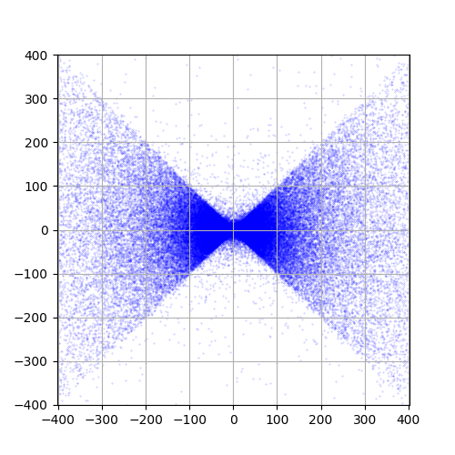
Say the user is interested in sampling a multivariate -stable random vector in dimension with , and whose spectral measure is uniform over the arcs and , that is, with probability 0.5, we draw a point uniformly on the arc , and with probability 0.5, we draw a point uniformly on the arc .
We assign equal probabilities to both arcs and the spectral measure of each arc is half the total measure of the sphere. Generally, the probability of each region is the ratio of the spectral measure of the region to the total mass of the sphere.
We create a class of the spectral measure sampler that we want by inheriting from the base class
BaseSpectralMeasureSampler. In the class that the user is creating, the function which samples the vectors in Theorem 1 should be provided. Moreover, the dimension of the desired alpha-stable vector and the total mass of the unit sphere should be specified. The created spectral measure sampler is then passed as an argument to thervs()method as shown in the following code.
The steps are presented below.
import aub_htp as ht
from aub_htp.random import BaseSpectralMeasureSampler
alpha = 0.3
shift= [0,0]
d = 2
n=500000

class ButterflySampler(BaseSpectralMeasureSampler):
    def sample(self, number_of_samples: int, random_state = None):
        p = np.random.rand(number_of_samples)
        theta = np.empty(number_of_samples)

        mask = p <= 0.5
        theta[mask] = np.random.uniform(-np.pi / 4, np.pi / 4, size=mask.sum())
        theta[~mask] = np.random.uniform(
            3 * np.pi / 4,
            5 * np.pi / 4,
            size=(~mask).sum()
        )

        x = np.cos(theta)
        y = np.sin(theta)

        return np.column_stack((x, y))

    def dimensions(self) -> int:
        return 2

    def mass(self) -> float:
        return 1.0

samples = ht.multivariate_alpha_stable.rvs(alpha = alpha, spectral_measure_sampler=ButterflySampler(), size = n, shift=shift)
We highlight that the mass of the sphere and the dimension should be specified when implementing the sub-class. The resulting scatter plot is shown in Figure 9b. It is important to emphasize that when , the custom spectral measure should satisfy the condition in equation (22).
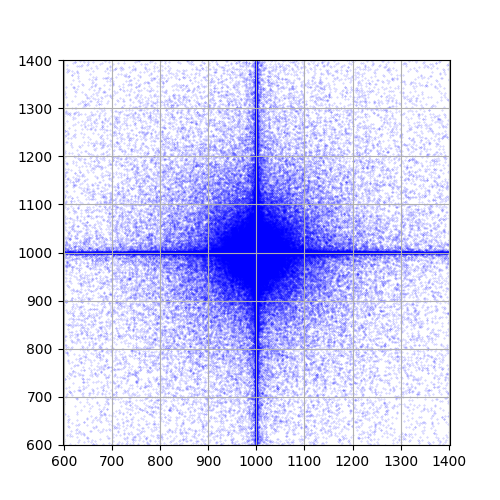
(a)Mix between isotropic and discrete spectral measures.
(b)A custom spectral measure
(c)Mix between custom and discrete spectral measures.
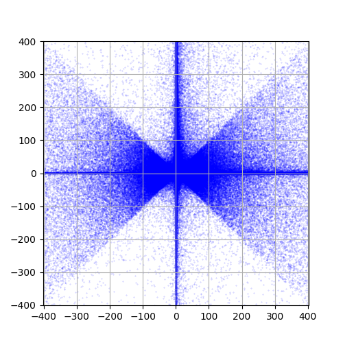
Figure 9:Scatter plots showing a custom spectral measure and different mixtures of spectral measures. The plots have been truncated to a range of 400 points within the shift vector.
One could mix a custom spectral measure, with another spectral measure. For example, we mix below equally the spectral measure defined above with the discrete spectral measure with and and the random vector has , .
import aub_htp as ht
from aub_htp.random import BaseSpectralMeasureSampler, DiscreteSampler, MixedSampler
alpha = 0.25
shift= [0,0]
d = 2
n=1000000
class ButterflySampler(BaseSpectralMeasureSampler):
    def sample(self, number_of_samples: int, random_state = None):
        p = np.random.rand(number_of_samples)
        theta = np.empty(number_of_samples)

        mask = p <= 0.5
        theta[mask] = np.random.uniform(-np.pi / 4, np.pi / 4, size=mask.sum())
        theta[~mask] = np.random.uniform(
            3 * np.pi / 4,
            5 * np.pi / 4,
            size=(~mask).sum()
        )

        x = np.cos(theta)
        y = np.sin(theta)

        return np.column_stack((x, y))

    def dimensions(self) -> int:
        return 2

    def mass(self) -> float:
        return 1.0

samples = ht.multivariate_alpha_stable.rvs(alpha = alpha, spectral_measure_sampler=ButterflySampler(), size = n, shift=shift)

# Discrete Spectral Measure
positions=[[1,0],[0,1],[-1,0],[0,-1]]
weights=[1,1,0.25,0.25]
sampler1 = DiscreteSampler(alpha = alpha, positions = positions, weights = weights)

#Spectral Measures and Their Associated Weights
spectral_measures=[sampler1, ButterflySampler()]
measure_weights=[0.5,0.5]

mixed_sampler=MixedSampler(spectral_measures=spectral_measures,weights=measure_weights)
samples = ht.multivariate_alpha_stable.rvs(alpha = alpha, spectral_measure_sampler = mixed_sampler,
shift = shift, size = n)
The resulting scatterplot is shown in Figure 9c.
6Conclusion
This paper presented AUB-HTP, a Python package for density computation and random variate generation of -stable distributions. The package is motivated by the practical difficulty of working with -stable laws, whose densities generally lack closed-form expressions and whose multivariate simulation requires careful handling of the underlying spectral measure.
AUB-HTP provides scalar density evaluation through a hybrid strategy that combines input standardization, Zolotarev-type integral representations, series formulas, and numerical inversion of characteristic functions. This design improves robustness across parameter regimes and enables systematic comparisons in terms of accuracy and runtime. The validation results show that the package provides reliable scalar density values and identify parameter regimes in which SciPy’s reference implementation appears to suffer from numerical inaccuracies.
The package also implements scalar and multivariate random variate generation. For multivariate -stable vectors, AUB-HTP uses LePage series representations and supports several spectral-measure models, including discrete, isotropic, sub-Gaussian/elliptical, mixed, and custom spectral measures. These features extend the range of -stable models that can be simulated within the Python ecosystem. The truncation-error analysis further provides guidance on the approximation induced by finite LePage-series representations.
By bringing together density evaluation, flexible simulation, validation, runtime analysis, and extensible implementation tools, AUB-HTP aims to make -stable modeling more accessible for computational work involving heavy-tailed data. Future developments may include multivariate PDF computation, CDF evaluation, parameter-estimation routines, further numerical acceleration, and application-oriented modules for communications, signal processing, and machine learning.
7Appendix: Error analysis for the LePage series estimate
In this appendix, we derive an upper bound on the mean square error of the LePage series estimate; we frequently use the following asymptotics of the gamma function from <i>NIST Digital Library of Mathematical Functions</i> (n.d.): Let and and be non-negative scalars. Since
then , there exists an such that
7.1The LePage series truncation error
The proof is as follows.
We start with the case . We have
which implies
where inequality is due to the Cauchy-Schwarz inequality. The equality in is due to the fact that , and , and inequality is due to (35). Inequality is due to the fact that
For the case , since , equation (22) implies . Let then we have
where equality is due to the fact that and is justified since , and , . The rest of the equalities and inequalities follow by similar steps as in the case .
One can clearly see that the bound on the error decays faster for smaller values of . This indicates that this sampling method can appropriately handle the difficult region of small values of .
7.2Sub-Gaussian error
Sampling a multivariate sub-Gaussian -stable vector can be done by first computing the truncated series for the isotropic spectral measure with unit-scale, and then applying where is the Cholesky decomposition of – the desired shape matrix as described in Section 4.2.3. The resulting MSE in that case satisfies
where we used the fact that , with –the largest eigenvalue of – being the norm of matrix Horn & Johnson (1985). Finally, one can upperbound using Theorem 2.
The characteristic function of a random variable is given by the expected value of , It uniquely determines the distribution of , and it always exists.
The term -stable is used to refer to the stable family excluding the Gaussian law.
- Nassar, M., Gulati, K., Sujeeth, A. K., Aghasadeghi, N., Evans, B. L., & Tinsley, K. R. (2008). Mitigating near-field interference in laptop embedded wireless transceivers. IEEE International Conference on Acoustics, Speech and Signal Processing, 1405–1408. 10.1109/ICASSP.2008.4517882
- Tsihrintzis, G. A., Tsakalides, P., & Nikias, C. L. (1995). Signal detection in severely heavy-tailed radar clutter. Conference Record of The Twenty-Ninth Asilomar Conference on Signals, Systems and Computers, 2, 865–869 vol.2. 10.1109/ACSSC.1995.540823
- Crovella, M. E., Taqqu, M. S., & Bestavros, A. (1998). Heavy-tailed probability distributions in the World Wide Web. A Practical Guide to Heavy Tails, 1, 3–26.
- Nolan, J. P. (2013). Multivariate elliptically contoured stable distributions: theory and estimation. Computational Statistics, 28(5), 2067–2089. 10.1007/s00180-013-0396-7
- Taleb, N. N. (2022). Statistical Consequences of Fat Tails: Real World Preasymptotics, Epistemology, and Applications. https://arxiv.org/abs/2001.10488
- B. V. Gnedenko and A. N. Kolmogorov. (1968). Limit Distributions for Sums of Independent Random Variables. Addison-Wesley Publishing Company.
- Chambers, J. M., Mallows, C. L., & Stuck, B. W. (1976). A Method for Simulating Stable Random Variables. Journal of the American Statistical Association, 71(354), 340–344.
- Zolotarev, V. M. (1986). One-Dimensional Stable Distributions (Vol. 65). American Mathematical Society.
- A. V. Skorohod. (1961). Asymptotic formulas for stable distribution laws. Selected Translations in Mathematical Statistics and Probability, 1, 157–161.
- Pollard, H. (1946). The Representation of \(e^-x^λ\) as a Laplace Integral. Bulletin of the American Mathematical Society, 52(10), 908–910. 10.1090/S0002-9904-1946-08608-2
- Bergström, H. (1952). On Some Expansions of Stable Distribution Functions. Arkiv För Matematik, 2(4), 375–378. 10.1007/BF02591503
- LePage, R., Woodroofe, M., & Zinn, J. (1981). Convergence to a Stable Distribution Via Order Statistics. The Annals of Probability, 9(4), 624–632.
- Samorodnitsky, G., & Taqqu, M. S. (2000). Stable non-Gaussian random processes : stochastic models with infinite variance (1st ed.). Chapman & Hall/CRC.
- Nolan, J. P. (2020). Univariate Stable Distributions: Models for Heavy Tailed Data (1st Edition 2020). Springer Nature.
- Wintner, A. (1941). The Singularities of Cauchy’s Distributions. Duke Mathematical Journal, 8, 678–681.